SUPPORT VECTOR MACHINE(SVM)

Figure 1: Support Vector Machine

What is SVM

An SVM is an instance of a supervised machine learning algorithm used in classification and regression. Using the created method, get the best hyperplane that will successfully separate classes. In two-dimensional space, this is just a line going through a plane and halving it into parts, each representing one class. Those points which are closest to the hyperplane and influence its position are called support vectors. The aim of the SVM is to maximize the margin between these support vectors and the hyper plane, ensuring that the model will have the best generalization capabilities.

Concept of SVM

SVMs are applied for both linear and nonlinear classification with the help of the so-called kernel trick. Kernel transforms the input data into a higher-dimensional space where it is possible for such a dataset not to be linearly separable in its original space. The common kernel functions are the linear, polynomial, and radial basis function kernels. However, this technique run by the corresponding algorithm is very robust and accurate and can operate in high dimensional attributes, hence finding a wide application area from image recognition to bioinformatics and text classification.

Reference: https://youtu.be/_L39rN6gz7Y?feature=shared

Scenario

Today you are going to determine the suitable amount of dosage needed to cure the disease. However, the disease can only be cured if the amount of dosage provided is suitable. You first plot the amount of dosage with the unit of (mg) on an axis

Figure 2: Example of dosage data

                                        

The data in red color indicates that the disease is not cured while the data in green on the other hand represents that this amount of dosage can cure the disease.

Figure 3: Example of dosage data

Within this situation, be it where we place the threshold to classify our data, a lot of misclassifications will occur. However, with the assistance of support vector machine (SVM), there is a solution to our problem.

Figure 4: Example of data

We calculate the y axis by powering the value of the dosage on the x-axis by 2 and through plotting data using both its value on its x and y-axis. A curve will appear and we are able to categorize the data by drawing the threshold in between the data with different categories. That's what support vector machine model does.

In the context of Support Vector Machine, there are several terminologies that build the concept and forge the foundation of this machine learning model, namely margins, hyperplane, support vectors and kernals which will be explained in detail as below.

1) Margins

The term margin refers to the distance between the data itself and the threshold. There are 2 types of margin in SVM, which are

• Maximal margin classifiers
• Soft margin classifiers

Maximal Margin Classifiers

Figure 5: Example of data

If we choose to apply the threshold that provides us the largest margin to make classifications, then we are applying the Maximal Margin Classifier.

Soft margin classifiers

Soft margin classifiers are applied to provide flexibility to our SVM by allowing misclassifications.

Figure 6: Example of data

Before we allow misclassifications, we select a threshold that was very sensitive to the training data. In this condition, the bias is low and will result in poor performance when a new data is obtained.

Figure 7: Example of data

However, once we pick a threshold that was less sensitive to the training data and allowed misclassifications to happen. The bias would be higher and would result in a better performance when the model receives a new data.

Once we allow misclassifications, the distance between the data and the threshold is called soft margin and through applying the soft margin to determine the location of the threshold, we are applying the Soft Margin Classifier to classify the data.

In short, these support vector classifiers have the ability to handle outliers and overlapping classifications as they allow misclassifications to occur while training the model.

2) Hyperplane

A hyperplane is also known as a flat affine subspace or in simpler term, the threshold that separates the data.

Figure 8: Example of mass data

                                        

When the data is presented in 1-Dimensional, the hyperplane is a single point on the 1-Dimentional number line. That point is a "flat affine 0-Dimensional subspace".

Figure 9: Example of data in 2D

                                           

When the data is presented in 2-Dimensions, the hyperplane is a 1-Dimensional line in a 2-Dimensional space. The line is called a "flat affine 1-Dimensional subspace".

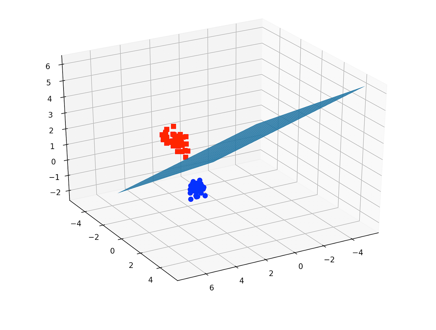Figure 10: Example of data in 3D

When the data is presented in 3-Dimensions, the hyperplane is a 2-Dimensional platform in a 3-Dimensional space. The platform is called a "flat affine 2-Dimensional subspace".

If the data is presented in 4-Dimensions and above, the support vector classifier is called hyperplane.

3) Support vectors

Every data in SVM is considered a vector but only those that are within a certain amount of range from the threshold are called as support vectors as it is these data that determines the position of the threshold.

Figure 11: Example of mass data

                                           

In a 1-Dimension, the data that lies on the edge and within the soft margin are called support vectors.

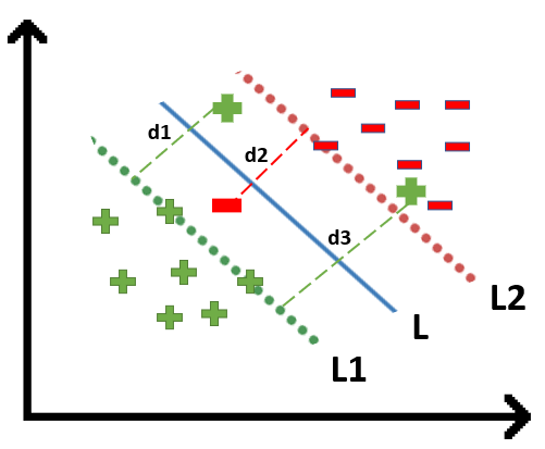Figure 12: Example of data

In a 2-Dimension, the data that lies within the range of L1 and L2 are called as support vectors.

4) Kernals

Kernals defines the relationship that is applied upon our data to find the support vector classifier. The mostly common used kernals are polynomial kernal and radial basis function kernal.

Polynomial Kernel

The formula of polynomial kernal can be concluded as

 (a x b + r) ^d

In which

a/b = 2 different observations in the dataset

r = coefficient of the polynomial

d = degree of the polynomial ( If d =1, the kernal computes the relationship between each pair of observations in 1-Dimension)

Through using this formula, we can obtain

• The high-dimensional coordinates for the data
• High dimensional relationships

The high-dimensional coordinates can be obtained through the dot product

(assuming the value of  r = 1/2 and d=2)

(a x b + 1/2)^2 

= (a x b + 1/2)(a x b + 1/2)

= ab + a^2b^2 + 1/4

= (a,a^2,1/2) . (b,b^2,1/2 )

First term = x-axis coordinates

Second term = y-axis coordinates

Third term = z-axis coordinates (if same can ignore)

The high-dimensional relationships can be obtain through plugging the values into the kernal.

Radial Basis Function (RBF) Kernel

RBF kernal classify the data depends on its surrounding data.

Figure 13: Example of data

                                 

For this scenario, since the surrounding data are classified as negative ( red color), then the new data (black color) are classified as negative as well.

The formula for RBF can be presented in 

Figure 14: Formula of RBF Kernel

y (gamma) = determined by Cross Validation, scales the squared distance which at the same time, scales the influence one observation has on another. Try an error until you get the best performance then use the value for the y.

(a - b)^2 = The squared distance between the 2 observations 

Hence, we can conclude that, the further 2 observations are from each other, the less influence they have on each other. The closest observations have a lot of influence on how the model classify the new observation

Parameters that you can tune for SVM

Kernel cache

Specifies how much memory is allocated for the cache of the Kernel matrix. It can significantly improve computational efficiency to set this large enough to hold the Kernel matrix in memory. However, it increases the memory footprint.

C

It is a regularization parameter that states the trade-off between achieving a low error on the train sample and minimizing the norm of the weights. The value of C is small, leading to a large margin with some misclassifications, and it is large, leading to a small margin with few misclassifications.

Epsilon for convergence

The tolerance for the optimization algorithm, thus specifying its stopping criterion. If the change of the objective value is smaller than the set Epsilon value, the algorithm would stop running. Smaller precision values of Epsilon bring a higher precision but at a higher number of iterations.

Maximum iterations 

This is the prespecified maximum number of iterations that the algorithm goes through. If the iterations that the algorithm goes through are more than the maximum iterations, then the algorithm is terminated, regardless of the fact that the required convergence standards are achieved or not. 

Scale

There has to be a scaling of the data before the SVM algorithm can be executed. 

L pos

It is the loss weight for samples in the positive class. This allows one to set cases of penalizing the mistake of an incorrect classification of a positive sample with a different penalty since it allows settings in a class that can counter problems related to imbalanced data.

Lneg

The loss weight of the positive class samples, and this gives the opportunity for the model to provide a different penalty for the misclassification of the negative samples.

Epsilon

Indicates within which epsilon tube no penalty is associated with the loss function during training. This defines a margin of tolerance where no penalty is given to errors.

Epsilon plus

A positive deviation from the actual values within which the prediction is considered acceptable.

Epsilon minus

Deviation from the actual values in which prediction is considered to be acceptable.

Cost balance

Balances the cost of misclassification across different classes. It becomes very useful for working with imbalanced datasets where one class is much more frequent than the other.

SVM Quadratic loss pos

Misclassification of the positive instances is quadratically penalized by the distance from the separating hyperplane. 

Quadratic loss neg

The penalty of negative misclassification increases quadratically, relative to the distance from the decision boundary. 

Kernal types

As mentioned, SVM can be implemented using various kernals. The list of all the kernal implementable with SVM includes

1. Dot: This is the simplest kernel that provides a representation of the dot product of two vectors. It linearly separable data so decision boundary is a straight line or hyper plane in higher dimensions.
2. Radial Basis Function Kernel (RBF Kernel): Maps data into an infinite dimensional space. It works in cases when the relation between class labels and attributes is nonlinear. 
3. Polynomial Kernel: The kernel representing the similarity in a polynomial feature space and it separates data non-linearly.
4. Neural or Sigmoid Kernel: This kernel is applied in problems where the relation of classes from each other is complicated. 
5. ANOVA (Analysis of Variance) Kernel: This kernel calculates the variance among various groups or categories so problems related to regression can be solved effectively. 
6. Epanechnikov Kernel: Mainly used for density estimation purposes and it is less common in support vector machines, while in kernel density estimation it can be used to smooth data in a non-parametric way.
7. Gaussian Combination Kernel: The kernel combines a few Gaussians that generalizes the flexibility of having multiple Gaussians with different parameters to be used and fit the structure of the data better.
8. Multiquadric Kernel: It belongs to the radial basis function kernels and it can be used in interpolation problems and in particular in geo-statistics. 

Implementation of SVM in python

Import the dataset 

Figure 15: Importing dataset

Getting a preview of the dataset

Figure 16: Head of dataset

Figure 17: Dataset overview

Checking dataset completeness

Figure 18: Code to check empty value

Figure 19: Total empty values

Data transformation using OrdinalEncoder

Figure 20: OrdinalEncoder

Understanding the correlation between features

Figure 21: Code to generate heatmap 

Figure 22: Heatmap

Splitting the data into training and testing

Figure 23: Splitting the dataset

Splitting the data and implement decision tree model

Figure 24: Implementing SVM

Test model performance

Figure 25: Get Accuracy Score

Figure 26: Model Accuracy

Advantages and disadvantages of SVM

Advantages 

1. Effective in High-Dimensional Spaces:

   • SVM is able to perform excellently in scenarios where the amount of dimensions exceeds the number of samples as they are particularly effective in high-dimensional spaces, making them suitable for text classification and other tasks with a large number of features.

2. Memory Efficiency:

   • SVM uses only a subset of the training points in the decision function known as the support vectors of the model, hence becoming memory efficient. This comes extremely useful while dealing with large data-sets.

3. Versatility:

   • SVM can be used whether it would be the task of linear or non-linear classification because complex relationship between features is easily handled by kernel functions such as polynomial, RBF, or sigmoid.

Disadvantages 

1. Computational Complexity:

   • Training SVMs can become quite computationally intensive, especially for large datasets. In most cases, training complexity is either quadratic or cubic in the number of samples, making this algorithm, in most cases, impractical for really large datasets.

2. Choice of Kernel:

   • Good performance in SVM depends much on the choice of the kernel function and its associated parameters. Choosing the right kernel, then, and tuning its parameter can only be indicative and requires domain knowledge and experimentation.

3. Memory Consumption:

   • While support vector machines are memory efficient in terms of prediction time, the training time can get really memory-consuming, mostly for large datasets, since it involves storing and processing large matrices.

Implementation of SVM in real life

1. Finance

Figure 27: Finance

• Third-party applications of SVMs like FICO also carry out fraud detection in banks, credit card companies, and other financial institutions. It does this by first analyzing patterns of transactions to loosely sort out outliers that could represent fraud, then makes use of the transactions data in determining the creditworthiness of people based on the analysis of their historical data to project propensity to default.

2. Healthcare

Figure 28: Healthcare

• Other health care organizations and even IBM Watson Health, along with research institutions, use them for diagnosis. However, SVM classifies medical images, like MRI, in order to point out the existence of any tumor or abnormality, or analyzes patient data to predict the response for various kinds of treatment and helps in designing personalized kind treatment plans.

3. Manufacturing and Quality Control

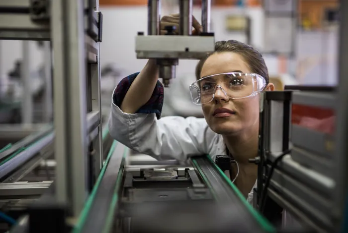Figure 29: Manufacturing and Quality Control

• Manufacturing companies like General Electric use SVM for fault detection in production processes. For example, an SVM can examine data derived from sensors and recognize irregularities in products as well as prediction of equipment failures from operational data so that seasonal corrective actions may be taken in advance, consequently reducing works' idle time.