AdaBoost This blog post will provide you with a comprehensive overview of Adaboost, exploring the theory behind this probabilistic algorithm and demonstrating its implementation using Python libraries. Dive in to uncover the advantages and disadvantages of neural network, as well as its real-world applications across various domains. With that, enjoy your journey in QDO! What is Adaboost AdaBoost (Adaptive Boosting) is an ensemble learning technique that combines multiple weak classifiers (often decision trees) to create a strong classifier. It works by training the weak classifiers sequentially, giving more weight to misclassified instances at each step so that subsequent classifiers focus more on the harder cases. The final prediction is made by combining the weighted votes of all weak classifiers. AdaBoost is effective at reducing bias and variance, and it’s particularly good for binary classification problems. However, it can be sensitive to noisy data and outliers. Concepts o...
LOGISTIC REGRESSION
 |
| Figure 1: Logistic regression |
This blogpost will provide you an overview of logistic regression, the theory behind the algorithm of logistic regression and its implementation using python libraries. Dive in to discover the advantages and disadvantages of logistic regression as well as its real life applications. With that, enjoy your journey in QDO.
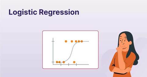
WHAT IS LOGISTIC REGRESSION
 |
| Figure 2: Logistic regression |
Logistic regression is considered as one of the most commonly used machine learning algorithm in the field of data science and it is used as a predictive model to predict the outcome base on the input variables feed into the model. This model is most suitable for binary classification tasks in which the dependent variable is categorical and typically represents two classes.
For example:
- yes/no
- 0/1
- true/false
The visualization of the results of logistic regression would be a graph with a line that is in form of the shape of S, which is what makes logistic regression analysis differs from other models.
Concept of logistic regression
Scenario
Lets say that we are trying to predict whether the a person is obese or not. We put the weight on our X-axis as in this scenario it is considered as our independent variable. As for the Y axis, our dependent variable is the status of the patient, whether that person is considered as obese or not.
As mentioned, the output of logistic regression would be in categorical value so for this scenario, the records that are not obese are classified as 0 and the records that are obese are classified as 1 within the Y-axis. The final graph would result in something as below.
 |
| Figure 3: Sample picture of scenario data |
The scenario above displays the result of a simple logistic regression model by predicting whether the person is obese or not solely on the weight variables.
However, in real life it is very seldom that the outcome of the prediction depends solely on one variable. Hence, more complicated model of logistic regression will be implemented such as determining whether the person is obese base on the person’s age and gender as well
What’s plotted in the X axis would not only be weight but instead weight + age + gender.
If you’re wondering how do we know if that particular variable is useful or not in predicting the obesity, we can try to include the variable within the X axis as well. In the event we want to know whether a person’s zodiac would impact the result of the analysis. Then our X value would be
weight + gender + age + zodiac
However, as we all know the zodiac of the patient is not related to the obese of a person so the result would yield no difference. Thus proving the fact that the zodiac is not a useful variable in predicting the obesity.
 |
| Figure 4: Logistic regression formula |
The figure above display the formula for logistic regression. Although it might seem complicated, the important parts of the formula are explained as below.
Coefficients
Coefficients is significant in determining the significance of a particular attribute towards the outcome of the analysis and the relationship between the input and the dependent variable.
The methods of getting the coefficient for logistic regression would differ base on the type of input variable
Coefficient for continuous variables
Using the formula log ((p/(1-p))), to get the y value for the new graph while the x-value remains the same.
p: the probability of the particular data within the logistic regression graph
 |
| Figure 5: Interpretation of data on a straight line |
The intersection of the straight line with the y axis is the coefficient.
The results would look something like this:
 |
| Figure 6: Coefficient result |
Intercept
Estimated Std: The y axis intercept, when the x value is 0, the y value would be -3.476
Error: the estimated error for the intercept
z value: Estimated Std / Error
Weight
Estimated Std: The gradient of the line drawn
Error: the estimated error for the gradient
z value: Estimated Std / Error
Coefficient for discrete variables
In terms of discrete variables , the way we measure the coefficient is different from the continuous variable but the first step remains the same.
 |
| Figure 7: Interpretation of discrete variable on a straight line |
Here’s where things started to get to differ, instead of drawing a straight line, we try to get the value of 2 variables which is
odds gene(normal)
= total normal gene that are within + Infinity / total normal gene that are within – Infinity
= 2/9
odds gene(mutated)
= total mutated gene that are within + Infinity / total mutated gene that are within – Infinity
= 7/3
The formula to determine the coefficient within this scenario are shown as below
| Figure 8: Formula of coefficients for discrete variable |
The final results of the coefficients would be something like this
 |
| Figure 9: Result of coefficients |
Intercept
Estimated Std: The value of log(odds gene(normal))
Error: the estimated error for the intercept for normal genes
z value: Estimated Std / Error
geneMutant
Estimated Std: The value of log(odds gene(mutated)) – log(odds gene(normal))
Error: the estimated error for the intercept for mutated genes
z value: Estimated Std / Error
Reference: https://youtu.be/vN5cNN2-HWE?feature=shared
Maximum Likehood
Maximum Likehood (MLE) applied in attempt to find the best-fitting coefficients that maximize the likelihood of the observed data.
In order to get the Maximum Likehood, we first implement the formula log ((p/(1-p))) to get this graph
 |
| Figure 10: Linear graph |
Next, proceed to plot each of the data on the drawn line and apply the formula below to convert the data back to the graph drawn in logistic regression.
 |
| Figure 11: Formula to convert linear graph to logistic regression graph |
Likehood in this extend refers to the probability of a record being marked as 1 or true for the dependent variable. If the record is marked as 0 or false for its dependent variable, we must use 1 to minus its probability before further calculation.
An example of the calculation of the likehood are demonstrated as below.
 |
| Figure 12: Likehood formula |
Proceed to rotate the straight line and repeat the process, the maximum likehood will be the maximum value of likehood obtain among all rotation of the line.
 |
| Figure 13:Rotation of graph |
Reference: https://youtu.be/BfKanl1aSG0?feature=shared
Implementation of logistic regression in python
Dataset source: https://www.kaggle.com/datasets/elikplim/car-evaluation-data-set
Importing libraries and dataset
import pandas as pd
data=pd.read_csv('car.data')
Overview of the dataset
data.head()

Ensuring that there are no missing values within the dataset
data.isna().sum()

Data preprocessing
data['doors']=data['doors'].replace('5more','5')
data['persons']=data['persons'].replace('more','5')
from sklearn.preprocessing import OrdinalEncoder
encoder=OrdinalEncoder()
data['buying']=encoder.fit_transform(data[['buying']])
data['maint']=encoder.fit_transform(data[['maint']])
data['lug_boot']=encoder.fit_transform(data[['lug_boot']])
data['safety']=encoder.fit_transform(data[['safety']])
data['class']=encoder.fit_transform(data[['class']])
Determining the dependent and independent variables
from sklearn.model_selection import train_test_split
X=data.drop('class',axis=1)
y=data['class']
Splitting the dataset into testing and training and applying the model
#import Logistic Regression
from sklearn.linear_model import LogisticRegression
lr=LogisticRegression()
X_train,X_test,y_train,y_test=train_test_split(X,y,test_size=0.2,random_state=42)
lr.fit(X_train,y_train)
Get prediction result
y_pred=lr.predict(X_test)
Get prediction accuracy
from sklearn.metrics import accuracy_score
print(accuracy_score(y_test,y_pred))
0.661849710982659
from sklearn.metrics import confusion_matrix
print(confusion_matrix(y_test,y_pred))

Parameters that you can tune in logistic regression
Solver
- decides the algorithm that will be used for optimization
- The types of solver available are mentioned as below
- AUTO - the software will automatically opt for the best solver.
- IRLSM - adjusts the weights of the logistic regression model based on the errors from the previous iteration
- L_BFGS - suitable for situations that contains large amount of variables
- COORDINATE_DESCENT_NAIVE - the algorithm will update each parameter one at a time
- COORDINATE_DESCENT - similar to COORDINATE_DESCENT_NAIVE but applies more complicated techniques to improve efficiency.
- GRADIENT_DESCENT_LH- the model parameters are updated iteratively in the direction of the negative gradient of the loss function.
- GRADIENT_DESCENT_SQERR- calculate the difference between predicted probabilities and actual outcomes and squared.
Reproducible
- the results achieved with the same data and parameters are always the same.
Use regularization
- prevent overfitting by penalizing large coefficients in the model
Early stopping
-stop training the model once the model's performance starts to drop.
Stopping rounds
-the number of iterations that the early stopping rule should wait before stopping the training process.
Stopping tolerance
- the threshold for measuring the new result against the greatest result to determine if training should stop.
Standardize
- the independent variables will be standardized before the training of the model commence.
Non-negative coefficients
- restrict the model to only have non-negative coefficients.
Add intercept
- Allow the model to fit the data better by adjusting the decision boundary.
Compute p-values
- Help in determining the statistical significance of each input variable's coefficient.
Remove collinear columns
- Cause the algorithm to identify and remove collinear columns from the dataset before training the model.
Missing values handling
- Determines the method use for handling missing values.
- The selection of this parameter includes
- MeanImputation - replace missing value with the mean value of the column
- Plugvalues -replace missing values with estimated values.
- Skip - ignore records with missing values entirely
Max iterations
- The maximum number of iterations the optimization algorithm should implement to obtain the best coefficients for the logistic regression model.
Max runtime seconds
- Sets the maximum allowed time in seconds for the model to run.
Penalty
- The parameter that will be used in the penalization of the algorithm
C
- The smaller the value, the stronger the regularization strength
Advantages and disadvantages of logistic regression
Advantages
- The results of logistic regression can be easily interpreted as the result is very straightforward. Hence it is easy to explain the result of the analysis to stakeholders or non-IT related clients.
- Logistic regression can be implemented easily as it doesn’t require a lot of computational resources and time compared to deep learning algorithms which makes this algorithm very beginner-friendly to those who are new to machine learning algorithms to implement.
- Understanding that this model provides probabilities as its output, it can be utilized for decision-making processes that require understanding of confidence levels in predictions.
Disadvantages
- Logistic regression assumes a linear relationship between the independent variables and the log-odds of the dependent variable. If the actual relationship is not linear, error in the analysis might occur
- Logistic regression falls short in capturing complex relationship between variables as the algorithm for logistic regression is too simple compared to decision trees or neural networks which can handle complex interactions better.
- Logistic regression can be sensitive to outliers, which can distort the results. It is compulsory to remove the outlier during the data preprocessing phase before implementing the logistic regression model.
Implementation of logistic regression in real life
Hotel Booking
 |
| Figure 14: Booked hotel room |
Booking.com has implemented a variety of machine learning algorithms throughout their entire website which includes predicting users’ intentions and recognizes human behavior.
Common questions include
- Where will you go?
- Where do you prefer to stop?
- What are you planning to do?
Before the user had even made their move, the prediction had been done and the system will guide the user to their desired action within the website. None of these would be accomplished without the implementation of logistic regression algorithm.
Credit scoring
 |
| Figure 15: Credit score |
ID Finance , a financial company that had been operating for decades implements logistic regression for credit scoring because this machine learning model is easily interpretable. This is suitable for their face-paced working environment as they can be asked by a regulator about a certain decision at any moment.
It is easy to find out which variables affect the final result of the predictions more and which ones less by implementing logistic regression so ID Finance optimizes its capability to find the optimal number of features and eliminate redundant variables with methods like recursive feature elimination.
Fraud Detection
 |
| Figure 16: Fraud detection |
Payment processing companies like PayPal use logistic regression to detect fraudulent transactions because as a company that emphasizes on payment transection, the security of the platform is above all else and would impact the reputation of the company. By applying logistic regression into their system, the model is able to analyze transaction patterns and flags those that are likely to be fraudulent based on historical fraud data.
Comments
Post a Comment